Particle Dynamics Models

Population balance models use an Eulerian description of particles, in which average properties of the particle population, such as number density, mass, and surface area, are treated as continuous quantities and tracked by solving scalar transport equations. These methods are computationally less expensive than mesoscale approaches, such as the discrete element method (DEM), and can be readily coupled with chemical kinetics in CFD solvers to simulate soot formation in laminar and turbulent configurations.

Omnisoot implements two particle dynamics models: a monodisperse population balance model (MPBM), which tracks four variables and therefore requires four transport equations, and a fixed-sectional population balance model (SPBM), which tracks three variables per section. In the SPBM, the total number of transport equations is equal to the number of tracked variables multiplied by the number of sections.

Tracking the total number concentrations of agglomerates and primary particles, together with the total carbon content of soot, enables the model to describe the evolving fractal-like morphology and surface area of soot agglomerates. These properties are required to calculate particle collision frequencies [7], as well as oxidation and surface-growth rates [8]. Tracking the hydrogen content of soot enables the model to represent soot composition and, consequently, its maturity [9] and surface reactivity [10].

The common features of the implemented particle dynamics models are reviewed in the Common Features section. The composition, expressed by the H/C ratio, diffusion coefficient, and morphology of soot particles are calculated in the same manner for the MPBM and for each section of the SPBM. However, the particle dynamics models differ in their treatment of coagulation and in how the contributions from inception, surface growth, and coagulation are processed to generate the source terms of the soot variables, \(S_{\varphi}\), used in the transport equations.

Common Features

Soot Morphology

The evolving fractal-like structure of soot agglomerates is characterized by the ratios of mobility diameter to primary-particle diameter, \(d_m/d_p\), and mobility diameter to gyration diameter, \(d_m/d_g\). These relationships can be described using power laws derived from mesoscale simulations.

Incipient soot initially consists of approximately spherical particles formed from PAHs. These particles grow through surface reactions and form agglomerates through coagulation. The particle collision frequency depends on the evolving fractal-like structure of the agglomerates [7].

The mobility and gyration diameters are calculated using power laws developed to describe soot morphology in premixed flames [11], diffusion flames [12], and diesel engines [13]. Fig. 4 shows a schematic of a soot agglomerate composed of 12 primary particles, with the primary-particle diameter, \(d_p\), mobility diameter, \(d_m\), and gyration diameter, \(d_g\), indicated.

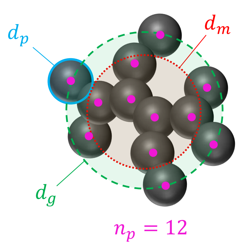
Fig. 4 Schematic of a soot agglomerate composed of 12 primary particles (\(n_p=12\)). The primary-particle diameter, \(d_p\), mobility diameter, \(d_m\), and gyration diameter, \(d_g\), are indicated.

The number of primary particles per agglomerate in section \(i\), \(n_p^i\), is obtained by dividing the number concentration of primary particles in section \(i\) by the number concentration of agglomerates in that section:

(22)\[n_p^i = \frac{N_{\mathrm{pri}}^i}{N_{\mathrm{agg}}^i}.\]

The primary-particle diameter, \(d_p^i\), is determined from the total carbon content and the number density of primary particles:

(23)\[d_p^i = \left[ \frac{6}{\pi} \frac{C_{\mathrm{tot}}^i W_{\mathrm{carbon}}}{\rho_{\mathrm{soot}}} \frac{1}{N_{\mathrm{pri}}^i Av} \right]^{1/3}.\]

The DEM-derived power laws [14] relate \(d_m^i\) and \(d_g^i\) to \(d_p^i\) and \(n_p^i\):

(24)\[d_m^i = d_p^i \left(n_p^i\right)^{0.45}.\]

(25)\[\begin{split}d_g^i = \begin{cases} \dfrac{d_m^i}{\left(n_p^i\right)^{-0.2}+0.4}, & n_p^i>1.5, \\[6pt] \dfrac{d_m^i}{1.29}, & n_p^i\leq 1.5. \end{cases}\end{split}\]

The collision diameter, \(d_c^i\), is defined as the larger of the mobility and gyration diameters:

(26)\[d_c^i = \max\left(d_m^i,d_g^i\right).\]

The volume-equivalent diameter, \(d_v^i\), is the diameter of a sphere with the same mass as the agglomerate:

(27)\[d_v^i = d_p^i \left(n_p^i\right)^{1/3}.\]

Assuming spherical primary particles, the surface area of a primary particle is

(28)\[A_p^i = \pi\left(d_p^i\right)^2.\]

For each section, \(A_{\mathrm{tot}}^i\) is defined as the total surface area of soot particles per unit mass of gas mixture:

(29)\[A_{\mathrm{tot}}^i = N_{\mathrm{pri}}^i Av A_p^i.\]

The mass of each agglomerate, \(m_{\mathrm{agg}}^i\), is expressed as

(30)\[m_{\mathrm{agg}}^i = \frac{C_{\mathrm{tot}}^i W_{\mathrm{carbon}}} {N_{\mathrm{agg}}^i Av}.\]

Soot Composition

The elemental carbon-to-hydrogen ratio, C/H, is used as a measure of soot maturity. It increases from \(\mathrm{C/H}<2\) for incipient soot [15], to \(2<\mathrm{C/H}<10\) for nascent soot [16], and to \(\mathrm{C/H}>20\) for mature soot [17].

Soot agglomerates are assumed to contain a pure-carbon graphitic core [9], with all hydrogen atoms located on the particle surface [10]. The C/H ratio is calculated from the total carbon and hydrogen contents:

(31)\[\left(\frac{C}{H}\right)^i = \frac{C_{\mathrm{tot}}^i}{H_{\mathrm{tot}}^i}.\]

In the SPBM, the carbon content of each agglomerate is predefined according to the section in which the agglomerate is located. In the MPBM, it is calculated by dividing \(C_{\mathrm{tot}}\) by \(N_{\mathrm{agg}}\). The hydrogen content of each agglomerate is calculated in both particle dynamics models as

(32)\[H_{\mathrm{agg}}^i = \frac{H_{\mathrm{tot}}^i}{N_{\mathrm{agg}}^i}.\]

Diffusion of Soot Particles

The diffusion coefficient of soot particles in section \(i\), \(D^i\), is calculated as

(33)\[D^i = \frac{k_B T}{f^i}.\]

Here, \(f^i\) is the friction coefficient of the particles in the gas mixture:

(34)\[f^i = \frac{3\pi\mu d_m^i}{C^i\left(d_m^i\right)}.\]

The Cunningham correction factor, \(C^i\), accounts for non-continuum effects in the transition and free-molecular regimes. For a particle of diameter \(d\), it is calculated as

(35)\[C^i(d) = 1 + \frac{2\lambda}{d} \left[ 1.21 + 0.4\exp\left( -\frac{0.78d}{\lambda} \right) \right].\]

Here, \(\lambda\) is the mean free path of the gas mixture:

(36)\[\lambda = \frac{\mu}{\rho} \sqrt{ \frac{\pi W_{\mathrm{gas}}} {2k_B Av T} }.\]

The mean free path is a property of the gas mixture and does not depend on particle mass or morphology.

Sectional Population Balance Model (SPBM)

A fixed-pivot sectional population balance model (SPBM) is used to describe particle dynamics [18]. The particle mass range is divided into discrete sections, each of which contains agglomerates of the same representative mass. Fig. 5 illustrates the interactions between the gas phase and the mass sections, as well as the mechanisms by which particles move between sections.

Inception introduces new particles into the first section with a mass corresponding to that of the incipient particle. Particles in each section can migrate to higher sections by gaining mass through surface growth and coagulation, and return to lower sections when they lose mass through oxidation. Fragmentation into smaller particles is not considered. Particles attach through point contact without coalescence.

The section masses are defined by a geometric progression whose initial value is equal to the mass of an incipient soot particle and whose common ratio is the sectional spacing factor, \(SF\). The representative mass of each section is approximated using the carbon content of agglomerates, expressed in moles:

(37)\[C_{\mathrm{agg}}^i = \frac{n_{c,\min}}{Av} SF^{i-1}.\]

Here, \(i-1\) is the exponent of \(SF\). The hydrogen mass is neglected when assigning agglomerates to sections.

The total number densities of agglomerates, \(N_{\mathrm{agg}}^i\), and primary particles, \(N_{\mathrm{pri}}^i\), together with the total hydrogen content, \(H_{\mathrm{tot}}^i\), are tracked in each section. Because the representative mass of each section is fixed, the total carbon content in section \(i\) can be calculated from the number of agglomerates:

\[C_{\mathrm{tot}}^i = N_{\mathrm{agg}}^i Av C_{\mathrm{agg}}^i.\]

The morphological properties of each section are calculated using the equations presented in the Soot Morphology section.

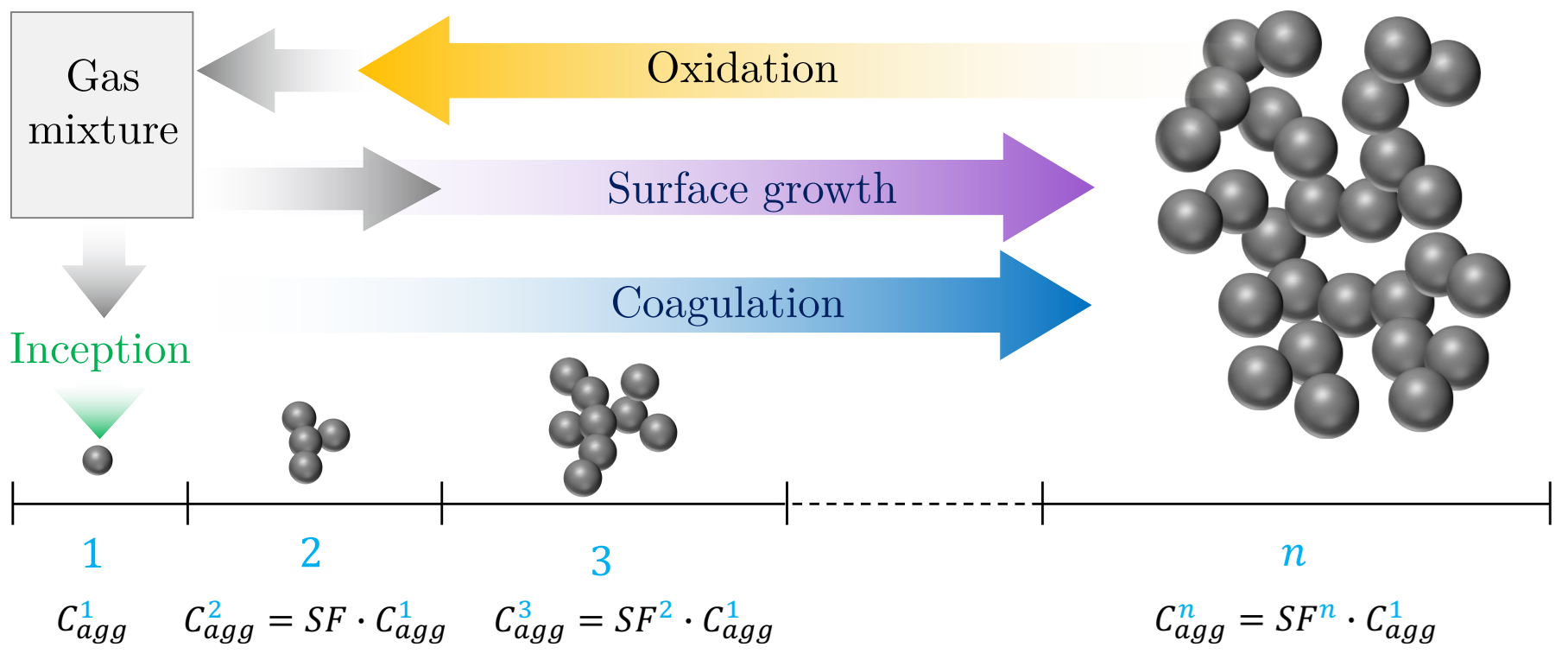
Fig. 5 Illustration of the sections used in the SPBM. The representative section masses increase geometrically according to the sectional spacing factor, \(SF\). Inception introduces new particles into the first section. Particles move to higher sections through coagulation and surface growth and return to lower sections through oxidation. Carbon and hydrogen are transferred from the gas phase to the particle phase through inception and surface growth and returned to the gas phase through oxidation.

New particles formed by coagulation are assigned to higher sections with a total mass equal to the sum of the masses of the colliding particles. If the mass of the resulting particle lies between two consecutive section masses, its contribution is distributed proportionally between those sections.

In some cases, the mass of a newly formed particle may exceed the upper bound of the last section and fall outside the tracked mass range. This can lead to mass loss, which is a known limitation of fixed-pivot sectional models [19]. The issue can be mitigated by choosing a sufficient number of sections and an appropriate spacing factor so that the uppermost sections remain unoccupied during the simulation.

In the SPBM, the source terms of the tracked soot variables appearing in Equations (5), (11), and (18) are divided into contributions from inception, surface growth and PAH adsorption, oxidation, and coagulation. The HACA surface-growth and PAH-adsorption contributions are combined under the subscript \(\mathrm{haca,ads}\) because both mechanisms increase particle mass. The source terms for section \(i\) are

(38)\[S_{N_{\mathrm{agg}}}^i = \left(S_{N_{\mathrm{agg}}}^i\right)_{\mathrm{inc}} + \left(S_{N_{\mathrm{agg}}}^i\right)_{\mathrm{haca,ads}} + \left(S_{N_{\mathrm{agg}}}^i\right)_{\mathrm{ox}} + \left(S_{N_{\mathrm{agg}}}^i\right)_{\mathrm{coag}}.\]

(39)\[S_{N_{\mathrm{pri}}}^i = \left(S_{N_{\mathrm{pri}}}^i\right)_{\mathrm{inc}} + \left(S_{N_{\mathrm{pri}}}^i\right)_{\mathrm{haca,ads}} + \left(S_{N_{\mathrm{pri}}}^i\right)_{\mathrm{ox}} + \left(S_{N_{\mathrm{pri}}}^i\right)_{\mathrm{coag}}.\]

(40)\[S_{H_{\mathrm{tot}}}^i = \left(S_{H_{\mathrm{tot}}}^i\right)_{\mathrm{inc}} + \left(S_{H_{\mathrm{tot}}}^i\right)_{\mathrm{haca,ads}} + \left(S_{H_{\mathrm{tot}}}^i\right)_{\mathrm{ox}} + \left(S_{H_{\mathrm{tot}}}^i\right)_{\mathrm{coag}}.\]

Coagulation Source Terms

Coagulation redistributes the total numbers of agglomerates and primary particles, as well as the total number of hydrogen atoms, among the sections. The partial coagulation source terms for \(N_{\mathrm{agg}}^i\), \(N_{\mathrm{pri}}^i\), and \(H_{\mathrm{tot}}^i\) are

(41)\[\begin{split}\begin{aligned} \left(S_{N_{\mathrm{agg}}}^i\right)_{\mathrm{coag}} &= \sum_{k=1}^{n_{\mathrm{sec}}} \sum_{j=k}^{n_{\mathrm{sec}}} \left( 1-\frac{\delta_{jk}}{2} \right) \eta_{ijk} \zeta^{jk} \beta^{jk} N_{\mathrm{agg}}^j N_{\mathrm{agg}}^k \\ &\quad - N_{\mathrm{agg}}^i \sum_{m=1}^{n_{\mathrm{sec}}} \zeta^{im} \beta^{im} N_{\mathrm{agg}}^m. \end{aligned}\end{split}\]

(42)\[\begin{split}\begin{aligned} \left(S_{N_{\mathrm{pri}}}^i\right)_{\mathrm{coag}} &= \sum_{k=1}^{n_{\mathrm{sec}}} \sum_{j=k}^{n_{\mathrm{sec}}} \left( 1-\frac{\delta_{jk}}{2} \right) \eta_{p,ijk} \eta_{ijk} \zeta^{jk} \beta^{jk} N_{\mathrm{agg}}^j N_{\mathrm{agg}}^k \\ &\quad - N_{\mathrm{pri}}^i \sum_{m=1}^{n_{\mathrm{sec}}} \zeta^{im} \beta^{im} N_{\mathrm{agg}}^m. \end{aligned}\end{split}\]

(43)\[\begin{split}\begin{aligned} \left(S_{H_{\mathrm{tot}}}^i\right)_{\mathrm{coag}} &= \sum_{k=1}^{n_{\mathrm{sec}}} \sum_{j=k}^{n_{\mathrm{sec}}} \left( 1-\frac{\delta_{jk}}{2} \right) \eta_{h,ijk} \eta_{ijk} \zeta^{jk} \beta^{jk} N_{\mathrm{agg}}^j N_{\mathrm{agg}}^k \\ &\quad - H_{\mathrm{tot}}^i \sum_{m=1}^{n_{\mathrm{sec}}} \zeta^{im} \beta^{im} N_{\mathrm{agg}}^m. \end{aligned}\end{split}\]

Here, \(\delta_{jk}\) is the Kronecker delta:

(44)\[\begin{split}\delta_{jk} = \begin{cases} 1, & j=k, \\ 0, & j\neq k. \end{cases}\end{split}\]

The collision frequency between sections \(j\) and \(k\), \(\beta^{jk}\), can be calculated from the harmonic mean of the continuum-regime value, \(\beta_{\mathrm{cont}}^{jk}\), and the free-molecular-regime value, \(\beta_{\mathrm{fm}}^{jk}\):

(45)\[\beta^{jk} = \frac{ \beta_{\mathrm{fm}}^{jk} \beta_{\mathrm{cont}}^{jk} }{ \beta_{\mathrm{fm}}^{jk} + \beta_{\mathrm{cont}}^{jk} }.\]

(46)\[\beta_{\mathrm{fm}}^{jk} = \sqrt{ \frac{\pi k_B T}{2} \left( \frac{1}{m_{\mathrm{agg}}^j} + \frac{1}{m_{\mathrm{agg}}^k} \right) } \left( d_c^j+d_c^k \right)^2.\]

(47)\[\beta_{\mathrm{cont}}^{ij} = \frac{2k_B T}{3\mu} \left( \frac{C^j}{d_m^j} + \frac{C^k}{d_m^k} \right) \left( d_c^j+d_c^k \right).\]

Alternatively, the collision frequency can be calculated using the Fuchs interpolation:

(48)\[\beta^{jk} = \beta_{\mathrm{cont}}^{ij} \left[ \frac{ d_c^j+d_c^k }{ d_c^j+d_c^k+2+\delta_r^{jk} } + \frac{ 8\left(D^j+D^k\right) }{ \bar{c}_r^{jk} \left(d_c^j+d_c^k\right) } \right]^{-1}.\]

Here, \(\delta_r^{jk}\) and \(\bar{c}_r^{jk}\) are the root-sum-square mean distance and velocity of the particles, respectively:

(49)\[\delta_r^{jk} = \sqrt{ \left(\delta_a^j\right)^2 + \left(\delta_a^k\right)^2 }.\]

(50)\[\bar{c}_r^{jk} = \sqrt{ \left(c^j\right)^2 + \left(c^k\right)^2 }.\]

The mean particle velocity, \(c^i\), and the mean particle displacement, \(\delta_a^i\), are calculated as

(51)\[c^i = \sqrt{ \frac{8k_B T} {\pi m_{\mathrm{agg}}^i} }.\]

(52)\[\delta_a^i = \frac{1} {d_c^i\lambda_a^i} \left[ \left( d_c^i+\lambda_a^i \right)^3 - \left( \left(d_c^i\right)^2 + \left(\lambda_a^i\right)^2 \right)^{3/2} \right] - d_c^i.\]

The agglomerate stopping distance, \(\lambda_a^i\), is defined as

(53)\[\lambda_a^i = \frac{8D^i}{\pi c^i}.\]

In Equation (41), \(\eta_{ijk}\) distributes newly formed agglomerates between two consecutive sections so that mass is conserved during coagulation [20]:

(54)\[\begin{split}\eta_{ijk} = \begin{cases} \dfrac{ C_{\mathrm{agg}}^{i+1} - C_{\mathrm{agg}}^{jk} }{ C_{\mathrm{agg}}^{i+1} - C_{\mathrm{agg}}^i }, & C_{\mathrm{agg}}^i \leq C_{\mathrm{agg}}^{jk} < C_{\mathrm{agg}}^{i+1}, \\[10pt] \dfrac{ C_{\mathrm{agg}}^i - C_{\mathrm{agg}}^{jk} }{ C_{\mathrm{agg}}^i - C_{\mathrm{agg}}^{i-1} }, & C_{\mathrm{agg}}^{i-1} \leq C_{\mathrm{agg}}^{jk} < C_{\mathrm{agg}}^i, \\[10pt] 0, & \text{otherwise}. \end{cases}\end{split}\]

Here,

\[C_{\mathrm{agg}}^{jk} = C_{\mathrm{agg}}^j + C_{\mathrm{agg}}^k.\]

Similarly, \(\eta_{p,ijk}\) in Equation (42) and \(\eta_{h,ijk}\) in Equation (43) adjust the numbers of primary particles and hydrogen atoms assigned to consecutive sections:

(55)\[\eta_{p,ijk} = \frac{ C_{\mathrm{agg}}^i }{ C_{\mathrm{agg}}^{jk} } \left( n_p^j+n_p^k \right).\]

(56)\[\eta_{h,ijk} = \frac{ C_{\mathrm{agg}}^i }{ C_{\mathrm{agg}}^{jk} } \left( H_{\mathrm{agg}}^j + H_{\mathrm{agg}}^k \right).\]

In Equation (41), \(\zeta^{jk}\) is the coagulation efficiency of soot particles in sections \(j\) and \(k\). A value of \(\zeta^{jk}=1\) indicates that every collision successfully forms a new agglomerate. Numerical models [21] and experimental evidence [22] show that the coagulation efficiency decreases substantially for particles smaller than 10 nm in the free-molecular regime, \(\mathrm{Kn}\gg10\), because their high kinetic energy can exceed the magnitude of the attractive forces [23].

The coagulation efficiency between two colliding particles is described by Narsimhan and Ruckenstein [21] as

(57)\[\zeta^{ij} = 1 - \left( 1+\frac{\Phi_0^{ij}}{k_B T} \right) \exp\left( -\frac{\Phi_0^{ij}}{k_B T} \right).\]

Here, \(\Phi_0\) is the potential-well depth, that is, the minimum interaction energy between two colliding particles. Hou et al. [24] calculated \(\Phi_0\) for soot particles ranging from 1 to 15 nm by accounting for attractive and repulsive interactions among their constituent carbon and hydrogen atoms. They proposed the following expression based on the reduced diameter, \(d_r^{jk}\), of the colliding particles:

(58)\[\Phi_0^{ij} = -6.6891\times10^{-23} \left(d_r^{jk}\right)^3 + 1.1244\times10^{-21} \left(d_r^{jk}\right)^2 + 1.1394\times10^{-20} d_r^{jk} - 5.5373\times10^{-21}.\]

(59)\[d_r^{jk} = \frac{ d_c^i d_c^j }{ d_c^i+d_c^j }.\]

Equation (58) is valid for \(d_r^{jk}\) between 1 and 7 nm. The coagulation efficiency is assumed to be unity for particles with a reduced diameter greater than 7 nm.

Inception, Surface-Growth, and Oxidation Source Terms

Inception introduces equal numbers of agglomerates and primary particles into the first section:

(60)\[\begin{split}\left(S_{N_{\mathrm{agg}}}^i\right)_{\mathrm{inc}} = \begin{cases} \dfrac{1}{Av} \dfrac{I_{N,\mathrm{inc}}} {C_{\mathrm{agg}}^i}, & i=1, \\[8pt] 0, & \text{otherwise}. \end{cases}\end{split}\]

(61)\[\begin{split}\left(S_{N_{\mathrm{pri}}}^i\right)_{\mathrm{inc}} = \begin{cases} \dfrac{1}{Av} \dfrac{I_{N,\mathrm{inc}}} {C_{\mathrm{agg}}^i}, & i=1, \\[8pt] 0, & \text{otherwise}. \end{cases}\end{split}\]

(62)\[\begin{split}\left(S_{H_{\mathrm{tot}}}^i\right)_{\mathrm{inc}} = \begin{cases} I_{H,\mathrm{inc}}, & i=1, \\ 0, & \text{otherwise}. \end{cases}\end{split}\]

Surface growth and PAH adsorption increase both the carbon mass and hydrogen content of agglomerates, thereby transferring them to higher sections. To conserve mass, the rate at which agglomerates are removed from the original section and added to the target section is calculated by dividing the carbon growth rate by the mass difference between adjacent sections:

(63)\[\begin{split}\left(S_{N_{\mathrm{agg}}}^i\right)_{\mathrm{haca,ads}} = \frac{1}{Av} \begin{cases} -\dfrac{ I_{C_{\mathrm{tot}},\mathrm{haca}}^i + I_{C_{\mathrm{tot}},\mathrm{ads}}^i }{ C_{\mathrm{agg}}^{i+1} - C_{\mathrm{agg}}^i }, & i=1, \\[12pt] \dfrac{ I_{C_{\mathrm{tot}},\mathrm{haca}}^{i-1} + I_{C_{\mathrm{tot}},\mathrm{haca}}^{i-1} }{ C_{\mathrm{agg}}^i - C_{\mathrm{agg}}^{i-1} } - \dfrac{ I_{C_{\mathrm{tot}},\mathrm{haca}}^i + I_{C_{\mathrm{tot}},\mathrm{ads}}^i }{ C_{\mathrm{agg}}^{i+1} - C_{\mathrm{agg}}^i }, & 1<i<n_{\mathrm{sec}}, \\[12pt] \dfrac{ I_{C_{\mathrm{tot}},\mathrm{haca}}^{i-1} + I_{C_{\mathrm{tot}},\mathrm{ads}}^{i-1} }{ C_{\mathrm{agg}}^i - C_{\mathrm{agg}}^{i-1} }, & i=n_{\mathrm{sec}}. \end{cases}\end{split}\]

As agglomerates move between sections, they carry their primary particles and hydrogen atoms. Therefore, the agglomerate transfer rates are multiplied by \(n_p^i\) and \(H_{\mathrm{agg}}^i\), respectively:

(64)\[\begin{split}\left(S_{N_{\mathrm{pri}}}^i\right)_{\mathrm{haca,ads}} = \frac{1}{Av} \begin{cases} -\dfrac{ I_{C_{\mathrm{tot}},\mathrm{haca}}^i + I_{C_{\mathrm{tot}},\mathrm{ads}}^i }{ C_{\mathrm{agg}}^{i+1} - C_{\mathrm{agg}}^i }, & i=1, \\[12pt] \dfrac{ I_{C_{\mathrm{tot}},\mathrm{haca}}^{i-1} + I_{C_{\mathrm{tot}},\mathrm{ads}}^{i-1} }{ C_{\mathrm{agg}}^i - C_{\mathrm{agg}}^{i-1} } n_p^{i-1} - \dfrac{ I_{C_{\mathrm{tot}},\mathrm{haca}}^i + I_{C_{\mathrm{tot}},\mathrm{ads}}^i }{ C_{\mathrm{agg}}^{i+1} - C_{\mathrm{agg}}^i } n_p^i, & 1<i<n_{\mathrm{sec}}, \\[12pt] \dfrac{ I_{C_{\mathrm{tot}},\mathrm{haca}}^{i-1} + I_{C_{\mathrm{tot}},\mathrm{ads}}^{i-1} }{ C_{\mathrm{agg}}^i - C_{\mathrm{agg}}^{i-1} } n_p^{i-1}, & i=n_{\mathrm{sec}}. \end{cases}\end{split}\]

(65)\[\begin{split}\left(S_{H_{\mathrm{tot}}}^i\right)_{\mathrm{haca,ads}} = \frac{1}{Av} \begin{cases} -\dfrac{ I_{C_{\mathrm{tot}},\mathrm{haca}}^i + I_{C_{\mathrm{tot}},\mathrm{ads}}^i }{ C_{\mathrm{agg}}^{i+1} - C_{\mathrm{agg}}^i } H_{\mathrm{agg}}^i + I_{H_{\mathrm{tot}},\mathrm{haca}}^i + I_{H_{\mathrm{tot}},\mathrm{ads}}^i, & i=1, \\[12pt] \dfrac{ I_{C_{\mathrm{tot}},\mathrm{haca}}^{i-1} + I_{C_{\mathrm{tot}},\mathrm{ads}}^{i-1} }{ C_{\mathrm{agg}}^i - C_{\mathrm{agg}}^{i-1} } H_{\mathrm{agg}}^{i-1} - \dfrac{ I_{C_{\mathrm{tot}},\mathrm{haca}}^i + I_{C_{\mathrm{tot}},\mathrm{ads}}^i }{ C_{\mathrm{agg}}^{i+1} - C_{\mathrm{agg}}^i } H_{\mathrm{agg}}^i + I_{H_{\mathrm{tot}},\mathrm{haca}}^i + I_{H_{\mathrm{tot}},\mathrm{ads}}^i, & 1<i<n_{\mathrm{sec}}, \\[12pt] \dfrac{ I_{C_{\mathrm{tot}},\mathrm{haca}}^{i-1} + I_{C_{\mathrm{tot}},\mathrm{ads}}^{i-1} }{ C_{\mathrm{agg}}^i - C_{\mathrm{agg}}^{i-1} } H_{\mathrm{agg}}^{i-1} + I_{H_{\mathrm{tot}},\mathrm{haca}}^i + I_{H_{\mathrm{tot}},\mathrm{ads}}^i, & i=n_{\mathrm{sec}}. \end{cases}\end{split}\]

Similarly, agglomerates lose carbon mass through oxidation and move to lower sections while carrying their primary particles and hydrogen atoms:

(66)\[\begin{split}\left(S_{N_{\mathrm{agg}}}^i\right)_{\mathrm{ox}} = \frac{1}{Av} \begin{cases} \dfrac{ I_{C_{\mathrm{tot}},\mathrm{ox}}^{i+1} }{ C_{\mathrm{agg}}^{i+1} - C_{\mathrm{agg}}^i } - \dfrac{ I_{C_{\mathrm{tot}},\mathrm{ox}}^i }{ C_{\mathrm{agg}}^i }, & i=1, \\[12pt] \dfrac{ I_{C_{\mathrm{tot}},\mathrm{ox}}^{i+1} }{ C_{\mathrm{agg}}^{i+1} - C_{\mathrm{agg}}^i } - \dfrac{ I_{C_{\mathrm{tot}},\mathrm{ox}}^i }{ C_{\mathrm{agg}}^i - C_{\mathrm{agg}}^{i-1} }, & 1<i<n_{\mathrm{sec}}, \\[12pt] -\dfrac{ I_{C_{\mathrm{tot}},\mathrm{ox}}^i }{ C_{\mathrm{agg}}^i - C_{\mathrm{agg}}^{i-1} }, & i=n_{\mathrm{sec}}. \end{cases}\end{split}\]

(67)\[\begin{split}\left(S_{N_{\mathrm{pri}}}^i\right)_{\mathrm{ox}} = \frac{1}{Av} \begin{cases} \dfrac{ I_{C_{\mathrm{tot}},\mathrm{ox}}^{i+1} }{ C_{\mathrm{agg}}^{i+1} - C_{\mathrm{agg}}^i } n_p^{i+1} - \dfrac{ I_{C_{\mathrm{tot}},\mathrm{ox}}^i }{ C_{\mathrm{agg}}^i }, & i=1, \\[12pt] \dfrac{ I_{C_{\mathrm{tot}},\mathrm{ox}}^{i+1} }{ C_{\mathrm{agg}}^{i+1} - C_{\mathrm{agg}}^i } n_p^{i+1} - \dfrac{ I_{C_{\mathrm{tot}},\mathrm{ox}}^i }{ C_{\mathrm{agg}}^i - C_{\mathrm{agg}}^{i-1} } n_p^i, & 1<i<n_{\mathrm{sec}}, \\[12pt] -\dfrac{ I_{C_{\mathrm{tot}},\mathrm{ox}}^i }{ C_{\mathrm{agg}}^i - C_{\mathrm{agg}}^{i-1} } n_p^i, & i=n_{\mathrm{sec}}. \end{cases}\end{split}\]

(68)\[\begin{split}\left(S_{H_{\mathrm{tot}}}^i\right)_{\mathrm{ox}} = \frac{1}{Av} \begin{cases} \dfrac{ I_{C_{\mathrm{tot}},\mathrm{ox}}^{i+1} }{ C_{\mathrm{agg}}^{i+1} - C_{\mathrm{agg}}^i } H_{\mathrm{agg}}^{i+1} - \dfrac{ I_{C_{\mathrm{tot}},\mathrm{ox}}^i }{ C_{\mathrm{agg}}^i } H_{\mathrm{agg}}^i + I_{H_{\mathrm{tot}},\mathrm{ox}}^i, & i=1, \\[12pt] \dfrac{ I_{C_{\mathrm{tot}},\mathrm{ox}}^{i+1} }{ C_{\mathrm{agg}}^{i+1} - C_{\mathrm{agg}}^i } H_{\mathrm{agg}}^{i+1} - \dfrac{ I_{C_{\mathrm{tot}},\mathrm{ox}}^i }{ C_{\mathrm{agg}}^i - C_{\mathrm{agg}}^{i-1} } H_{\mathrm{agg}}^i + I_{H_{\mathrm{tot}},\mathrm{ox}}^i, & 1<i<n_{\mathrm{sec}}, \\[12pt] -\dfrac{ I_{C_{\mathrm{tot}},\mathrm{ox}}^i }{ C_{\mathrm{agg}}^i - C_{\mathrm{agg}}^{i-1} } H_{\mathrm{agg}}^i + I_{H_{\mathrm{tot}},\mathrm{ox}}^i, & i=n_{\mathrm{sec}}. \end{cases}\end{split}\]

Monodisperse Population Balance Model (MPBM)

The MPBM used in this study is based on the monodisperse model presented by Kholghy and Kelesidis [25]. It tracks \(N_{\mathrm{pri}}\), \(N_{\mathrm{agg}}\), \(C_{\mathrm{tot}}\), and \(H_{\mathrm{tot}}\). The coagulation model follows the same principles as the SPBM, but the calculations are greatly simplified by the monodispersity assumption. With well-justified assumptions, this approach has been shown to provide accuracy comparable to that of DEM and SPBM [8, 26].

The rate of decay of the agglomerate number concentration due to coagulation is

(69)\[I_{\mathrm{coag}} = -\frac{1}{2} \zeta \beta N_{\mathrm{agg}}^2.\]

Here, \(\zeta\) is the collision efficiency of agglomerates, calculated using Equation (57), and \(\beta\) is the collision frequency of agglomerates from the free-molecular regime, \(\mathrm{Kn}>10\), to the continuum regime, \(\mathrm{Kn}<0.1\).

In the transition regime, \(0.1<\mathrm{Kn}<10\), \(\beta\) can be calculated from the harmonic mean of the continuum-regime value, \(\beta_{\mathrm{cont}}\), and the free-molecular-regime value, \(\beta_{\mathrm{fm}}\). An enhancement factor of 1.82 is applied to account for the effect of polydispersity [27]:

(70)\[\beta = 1.82 \frac{ \beta_{\mathrm{fm}} \beta_{\mathrm{cont}} }{ \beta_{\mathrm{fm}} + \beta_{\mathrm{cont}} }.\]

(71)\[\beta_{\mathrm{fm}} = 4 \sqrt{ \frac{\pi k_B T}{m_{\mathrm{agg}}} } d_c^2.\]

(72)\[\beta_{\mathrm{cont}} = 8\pi d_m D.\]

Here, \(d_c\), \(D\), and \(m_{\mathrm{agg}}\) are calculated using Equations (26), (33), and (30), respectively.

Alternatively, \(\beta\) can be calculated using the Fuchs interpolation [28]:

(73)\[\beta = \beta_{\mathrm{cont}} \left[ \frac{ d_c }{ d_c+2\sqrt{2}\delta } + \frac{ 8D }{ \sqrt{2}c d_c } \right]^{-1}.\]

Here, \(c\), the mean particle velocity, and \(\delta\), the mean particle displacement, are calculated using Equations (51) and (52), respectively.

The source terms of the tracked variables combine the contributions from inception, surface growth, PAH adsorption, oxidation, and coagulation:

(74)\[S_{N_{\mathrm{agg}}} = \frac{ I_{N,\mathrm{inc}} }{ n_{c,\min} } + I_{\mathrm{coag}}.\]

(75)\[S_{N_{\mathrm{pri}}} = \frac{ I_{N,\mathrm{inc}} }{ n_{c,\min} }.\]

(76)\[S_{C_{\mathrm{tot}}} = I_{C_{\mathrm{tot}},\mathrm{inc}} + I_{C_{\mathrm{tot}},\mathrm{haca}} + I_{C_{\mathrm{tot}},\mathrm{ads}} - I_{C_{\mathrm{tot}},\mathrm{ox}}.\]

(77)\[S_{H_{\mathrm{tot}}} = I_{H_{\mathrm{tot}},\mathrm{inc}} + I_{H_{\mathrm{tot}},\mathrm{haca}} + I_{H_{\mathrm{tot}},\mathrm{ads}} - I_{H_{\mathrm{tot}},\mathrm{ox}}.\]